Excel is an amazing tool to record, manage, analyze data. It has many features that help you do advanced data analysis and reporting. Data entry can be a long and arduous task in Excel. But if you know the right tools and techniques, it can speed up your data entry and help ensure error-free work. Here are six data entry tips for Excel that will help get your work done faster: #1 – Use Drop Down Lists to Enter Data Quickly You can use a drop-down list in Excel to enter data from prespecified options. For example, if you have a list of names or products and you need to enter one of it in a range of cells, you can create a drop-down list with these names. Apart from speeding up data entry, drop down lists also ensure that the data entry is error free. Here are the steps to insert a drop-down list in a cell in Excel:
Select the cell or the range of cells in which you the drop down.
Go to the Data tab and click on the Data Validation option. In the Data Validation dialog box, within the Settings tab, select the ‘List’ option from the drop down. Specify the cells that have the items you want in the drop down (or manually enter it, separated by comma). Click OK.
This will add a drop down list to the selected cells. Now you can click
on the drop down icon, and it will show you the list of all the items. #2 – Use Fill Handle Fill handle makes it quick to enter data points that follow a pattern. For example, if you want to enter a sequence of numbers (such as 1,2,3..) in a column, you can do that quickly using the fill handle. Here are the steps to use fill handle in Excel:
Enter the data points in 2 consecutive cells. This will help fill handle in identifying the pattern. Select both the cells. Hover the mouse on the bottom end part of the selection. You will notice the cursor changes into a plus icon. Use the mouse left-click to drag the fill handle to cover the cells in which you want the entries done.
You can use fill handle in cases where Excel can recognize a pattern. For example, you can use it with numbers, month names (Jan, Feb, Mar..), years, day names (Mon, Tue, Wed..). #3 – Lock Rows/Columns Headers When you work with a lot of data in Excel, it could get difficult as you scroll away from the headers. While scrolling, the headers disappear and it sometimes makes it difficult to identify what a data point represents. Using Excel Freeze Panes option ensure that the headers are always visible. Here are the steps to lock the rows/columns headers in Excel:
Select the top left cell of the data set that does not include the headers.
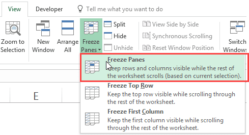
Go to the View tab and select Freeze Panes option (from the Freeze Panes drop-down).
Now when you scroll away to the right or the bottom, the headers will always be visible. #4 – Copy from the Cell Above Knowing useful Excel keyboard shortcuts can really help you speed up the work. One use keyboard shortcut is Control + D. It copies the content from the cell above it. This can come in handy in cases when you want to copy the cell right above it. #5 – Choose from a List of Already Entered Data When you are entering data points in a column, Excel gives you the option to select from the options that you have already entered. To get the list of options, select the cell and use the keyboard shortcut,
Alt + Down arrow key. As soon as you do this, it will show you the option in the cells above it. You can quickly select it and move to the next cell. Note that you will only see the list of unique items from cells that are right above/below the selected cell. If there are gaps between the selected cell and the ones with the data, it will not be shown. #6 – Quickly Move Through Multiple Worksheets When working with many worksheets, it may become quite irritating to use the mouse to sift through the worksheets. You can use the following keyboard shortcut to quickly move through the worksheets – Control + PageUp/PageDown. Control + PageUp will take you to the next worksheet and Control + PageDown will take you to the previous worksheet.


